Explicit Solvation

Solvation significantly affects the properties and reactivity of chemical systems. The inclusion of solvents in quantum chemical calculations is crucial for accurate predictions.

In another tutorial we covered implicit solvation, which involves including by default the solvent water in every WEASEL calculation. Implicit solvation provides a useful approximation of solvent effects for a given system. However, for a more complete understanding of solvent effects, explicit solvation is required.

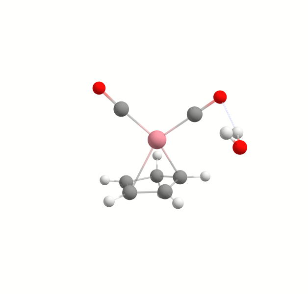
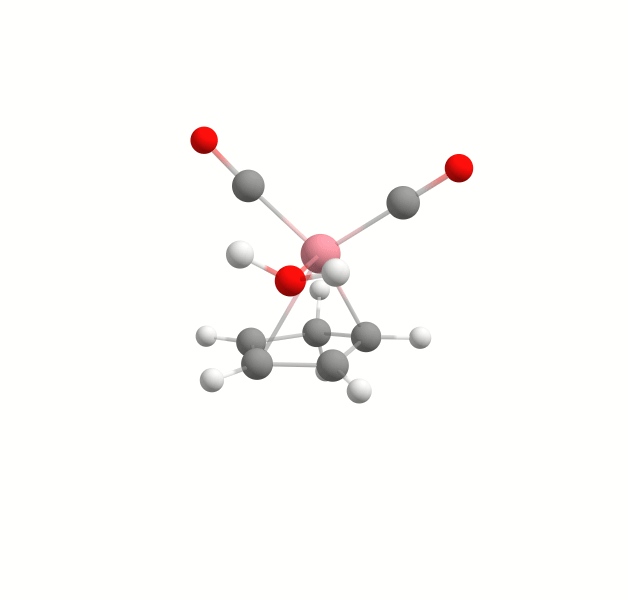
Explicit solvation is a method of computational chemistry in which solvent molecules are explicitly included in the calculation. It captures detailed solute-solvent interactions. There are several different approaches to explicit solvation. WEASEL offers two different options. The first option in WEASEL is stochastic explicit solvation, which treats the solvent molecules as a statistical ensemble surrounding the solute. The second option in WEASEL is docking explicit solvation using the Docker module, which positions solvent molecules at optimized interaction positions around the solute. The difference between these two approaches is illustrated below for the example of the cobalt complex [CpCo(CO)₂] in water.

Explicit solvation with the stochastic solvator.

Explicit solvation with the docking solvator.

In this tutorial we will explore how to incorporate explicit solvation into your WEASEL calculations. Both stochastic and docking approaches will be discussed. An additional WEASEL tool for explicit solvation is introduced, the Auto Solvator. It is an approach to automatically determine the number of solvent molecules strongly interacting with the solute. This allows to have a reasonable solute-solvent complex for different applications where explicit solvent molecules may play a role, but only the minimum number of explicit solvent molecules necessary should be included.

How to include explicit solvation in a WEASEL calculation

In this part of the tutorial we will focus on including explicit solvation in your WEASEL calculation. To include explicit solvation, all you have to do is add the keyword -solvent-expl to your input command:

weasel example.xyz -solvent-expl

By default, WEASEL simulations are run with the implicit solvent water. Water is also the default solvent used in explicit solvation, and the implicit solvent is still used in addition to explicit solvation. If you want to change your solvent, you can do so with the following command, here exemplarily shown for chloroform:

weasel example.xyz -solvent-expl -solvent chloroform

Note

A list of all solvents available in WEASEL can be found here.

You can also read an explicit solvent from a XYZ file by specifying it like this:

weasel example.xyz -solvent-expl chloroform.xyz

By default, the charge and multiplicity of each solvent molecule is zero and one. To change this, you can use the keywords -solvent-expl-charge N and -solvent-expl-mult N respectively.

Note

If you select your solvent from the list of available solvents in WEASEL using the -solvent keyword, the selected solvent will be used as the implicit and explicit solvent. However, when reading the explicit solvent via -solvent-expl, the implicit solvent is not changed. In such cases, unless explicitly specified with the -solvent keyword, the implicit solvent used is set to WEASEL's default, which is water.

If the keyword -solvent-expl is applied to your calculation, WEASEL will run through its basic workflow after the solvation process, as in a pre-optimization and optimization of the system together with its solvent, and then perform a single point DFT calculation. If you only want to apply explicit solvation to your system without any subsequent optimization steps, you can use the -solvent-expl-only argument:

weasel example.xyz -solvent-expl-only

You can add other operations or parameters to the command as needed. For example, to incorporate additional computational steps like conformational searches or spectral calculations, you can include the relevant keywords in your input command to perform the desired operations in the explicit solvent.

By default, stochastic explicit solvation is applied as it is less computationally demanding compared to docking solvation, which involves additional optimization steps. To use docking solvation utilizing a docking mechanism, which is explained in detail in another tutorial, you can specify the -solvent-expl-method docking argument:

weasel example.xyz -solvent-expl -solvent-expl-method docking

Note

Although the inclusion of explicit solvent molecules via the stochastic approach is not based on physical factors, it is not random and therefore the resulting solvent model is reproducible.

By default, one explicit solvent molecule is added to the model. However, to include additional solvent molecules, you can use the -solvent-expl-nsolv command line option when starting the WEASEL job. For example, the following input line initiates the addition of ten explicit solvent molecules to the model:

weasel example.xyz -solvent-expl -solvent-expl-nsolv 10

Note

By default, when you add multiple solvent molecules, they start to form a droplet around the solute. To disable this option you can use the keyword ``-solvent-expl-no-droplet''.

WEASEL output files

For a run in which -expl-solv is requested with no further workflow modification, the output file structure is as follows:

.
├── example.xyz
└── example
    ├── example.solvator.xyz
    ├── example_Opt.xyz
    ├── example.report
    ├── example.results.xyz
    ├── example.summary
    ├── BuildTopo
    │   └── example_BuildTopo job files
    ├── ExplicitSolvation
    │   └── example_ExplicitSolvation job files
    ├── PreOpt
    │   └── example_PreOpt job files
    ├── Opt
    │   └── example_Opt job files
    └── SP_DFT
        └── example_SP_DFT job files

Apart from the regular output files generated by WEASEL in the main directory, you will also find an additional file named example.solvator.xyz. This file shows the explicit solvent structure that has been constructed. It is important to note that this solvent order represents the output generated by the solvator. However, if subsequent optimization steps, such as a DFT optimization, are performed after solvation, the resulting solvent structure may be different. In such cases, you can find the corresponding final structure, including the changes from any additional calculation steps, in the usual example.results.xyz file.

Efficient solvent quantification with the WEASEL Auto Solvator

It is often unnecessary to include an excessive number of explicit solvent molecules in simulations. Instead, it may be more effective to focus on those that are strongly bound to the solute and thus can have a significant influence on its properties. Examples of cases where specifically bound solvent molecules may be relevant include spectroscopic properties, acidity (pKa values), catalysis in chemical or biological processes and many more. In WEASEL, the use of the Auto Solvator tool facilitates the identification of the minimum number of critical solvents. This allows us to focus our computational resources on the most relevant components of the system.

The Auto Solvator works by including solvent molecules in your simulation and calculating their interaction energy with the solute. Based on the interaction energy, it then distinguishes between solvent molecules that are strongly bound to the solute and those that have weaker or negligible interactions. The end result is a solute-solvent system with an optimized solvent structure, with the minimum number of solvent molecules in optimized positions and their corresponding interaction energies.

In the following section we provide a guide to running the Auto Solvator in WEASEL, explaining how it works and what results it produces.

Warning

Currently the Auto Solvator is only optimized for the solvent water. Use with other solvents is not recommended.

How to run a WEASEL Auto Solvator calculation

For the explanation and use of the Auto Solvator we will focus on the example of urea in water. If you want to do the calculation yourself, you can download for the XYZ coordinates file urea.xyz.

Once you have these coordinates ready, you can run the Auto Solvator using the following command:

$ weasel urea.xyz -solvent-expl-only -solvent-expl-nsolv auto

As you can see, no new WEASEL keywords are introduced in this context, but the already known keyword -solvent-expl-nsolv gets a new level of versatility. Instead of specifying a fixed number of solvent molecules, it is used here in conjunction with the term auto to automatically invoke the determination of the required solvent molecules.

To focus on only generating the minimal solvent-solute complex and indicating that no additional operations are required, it is advisable to pair with -solvent-expl-only. Altenatively you can also combine -solvent-expl-nsolv auto with other WEASEL keywords for succeeding calculations.

Steps of a WEASEL Auto Solvator calculation

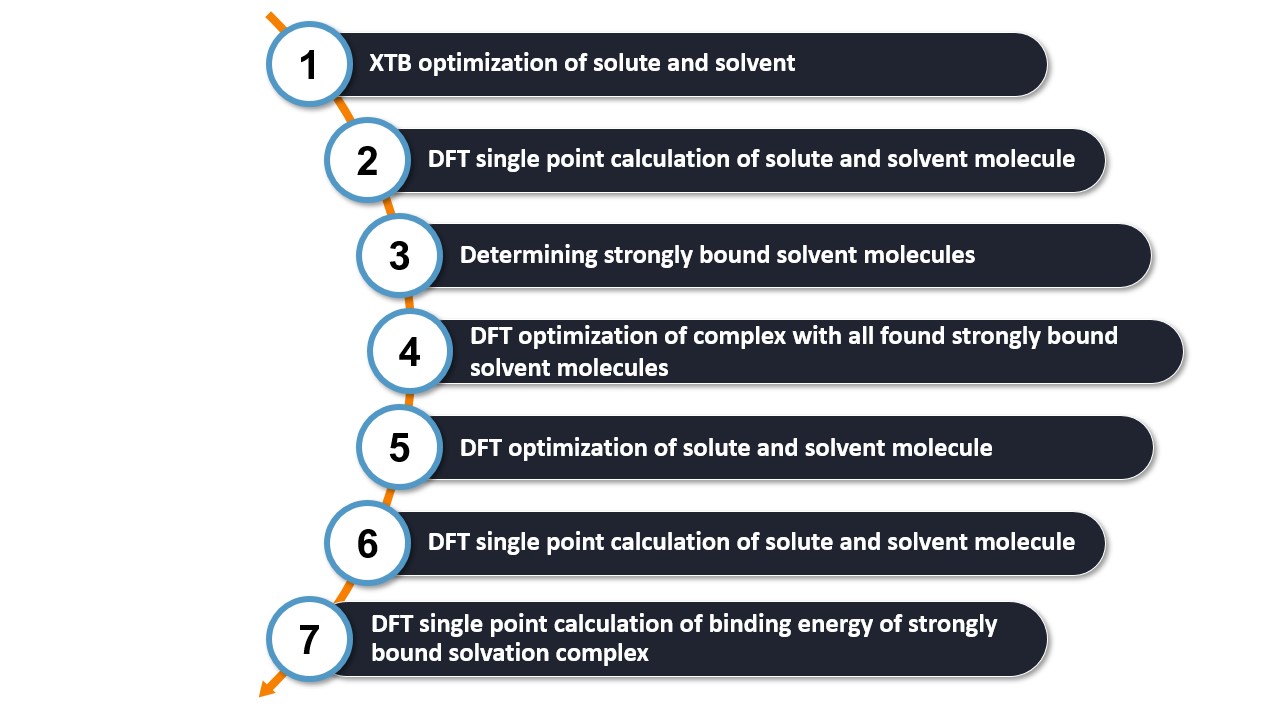
Step 1: Optimizing solute and solvent structures using XTB.

First, the solute and solvent structures are optimized at the XTB level. These optimized structures serve as the basis for the solvation model.

Step 2: Calculating SP-DFT energies for the solute and solvent using r2SCAN-3c.

A single point DFT calculation is performed using the r2SCAN-3c method on the in Step 1 optimized structures. The resulting energies are used for an initial evaluation of the binding energies in the solvation model in Step 3. This initial evaluation will help to determine whether a solvent molecule is strongly bound or not.

Step 3: Determining strongly bound solvent molecules for the solute.

Explicit solvent molecules are added to the in Step 1 optimized solute. Initially, either the square root of the number of atoms in the solute is added to the solvent molecules, or a minimum of five solvent molecules. The Auto Solvator applies the explicit solvation process using the docking scheme explained earlier, which performs the solvation process at the XTB level and strategically places solvent molecules in minimum energy positions around the solute.

After adding this set number of solvent molecules, the binding energy with the solute for each of the added solvent molecules is calculated. This involves calculating the single point energies with r2SCAN-3c of the solvent molecule together with the solute and subtracting the single point energies obtained in Step 2. If the resulting binding energy is less than or equal to -1.5 kcal/mol (a value determined through benchmarking with water and various molecules), the solvent molecule is classified as strongly bound; otherwise, it is not.

If any of the last three solvent molecules added is strongly bound, it indicates that additional solvent molecules may be needed to identify all the strongly bound water molecules and determine the minimal solute-solvent complex. Thus, a new cycle of five explicit solvent molecules is added to the model and their binding energy is calculated. This process is reiterated until all strongly bound solvent molecules are identified.

This step can be tracked in the report file, summarized with a table as demonstrated below using the urea example:

++++++++++++++++++++++++++++++++++++
| Summary: Added solvent molecules |
++++++++++++++++++++++++++++++++++++

Found a total of 5 strongly bound solvent molecules.
Threshold strongly bound: -1.500000 kcal/mol
#: Order in which solvent molecules were added.
+----+-----------------+------------------------+----------------+
| #  | Solvation cycle | Pair energy [kcal/mol] | Strongly bound |
+----+-----------------+------------------------+----------------+
| 1  |        1        |       -4.480725        |      yes       |
| 2  |        1        |       -1.816047        |      yes       |
| 3  |        1        |       -4.597790        |      yes       |
| 4  |        1        |       -3.100591        |      yes       |
| 5  |        1        |       -1.737940        |      yes       |
| 6  |        2        |       -0.339735        |       no       |
| 7  |        2        |       -0.544336        |       no       |
| 8  |        2        |       -0.179215        |       no       |
| 9  |        2        |       -1.089623        |       no       |
| 10 |        2        |       -0.404227        |       no       |
+----+-----------------+------------------------+----------------+

In this particular case, all water molecules added to urea in the initial solvation cycle exhibit strong binding. However, no strongly bound water molecules are discovered subsequently. The solvation process is thus concluded after two cycles, with a total of five strongly bound water molecules identified.

Step 4: Relaxing geometry of complex with all found strongly bound solvent molecules.

The solute-solvent complex, consisting only of the strongly bound solvent molecules determined in Step 3, undergoes geometry optimization at the r2SCAN-3c level. This process results in a more accurate structure of the final solute-solvent complex.

Step 5: Optimizing geometry of solute and solvent using r2SCAN-3c.

The geometry of the individual solute and solvent molecules from Step 1 is further optimized at the r2SCAN-3c level. This optimization provides a more reliable reference for the final binding energy calculation in Step 7.

Step 6: Calculating SP-DFT energies of solute and solvent using wB97X-V/def2-TZVP.

To improve energy accuracy, the energy of the optimized individual solute and solvent molecules from Step 5 is recalculated using wB97X-V/def2-TZVP.

Step 7: Calculating SP-DFT level binding energy of strongly bound solvation complex using wB97X-V/def2-TZVP.

In this final step, for each pair of strongly bound solvent molecules with the solute, the energy is recalculated at the wB97X-V/def2-TZVP level using the geometry obtained in Step 5. The final binding energy is then derived as the difference of the individual energies of the solute and solvent obtained in Step 6.

The binding energies are printed in the report file in order of binding strength, as shown for the urea example below:

+++++++++++++++++++++++++++++++++++
| Summary: Final binding energies |
+++++++++++++++++++++++++++++++++++
Pairs are sorted according to their binding energy.
#: Order in which solvent molecules were added.
+---+------------------------+
| # | Pair energy [kcal/mol] |
+---+------------------------+
| 3 |       -4.258085        |
| 1 |       -4.256883        |
| 4 |       -3.226972        |
| 2 |       -1.686766        |
| 5 |       -1.673672        |
+---+------------------------+

WEASEL output files and results

For a run in which the Auto Solvator is requested with no further modifications, the output file structure is as follows:

.
├── urea.xyz
└── urea
    ├── urea.report
    ├── urea.results.xyz
    ├── urea.summary
    ├── BuildTopo
    │   └── urea_BuildTopo job files
    └── ExplicitSolvation
        └── urea_ExplicitSolvation job files

The most important files and a brief description of their contents are listed in the table below.

File	Description
urea.results.xyz	Final optimized solute-solvent complex including the only strongly bound solvents
urea.report	Information about each step of the calculation, which solvent molecules are strongly bound to the solute, and the solvent-solute interaction energies
urea.summary	Summary of the results including the single point energies at the r2SCAN-3c level for all solute-solvent pairs and those at the wB97X-V level for all pairs with strongly bound solvent molecules as well as their pair binding energies

The structure in the urea.results.xyz file is that of the final solvent-solute complex. In this case it is urea with five strongly bound water molecules as shown below:

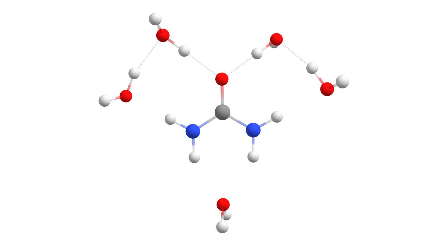
Final solute-solvent complex of urea with the number of strongly bound water molecules determined by the WEASEL Auto Solvator.

Keywords and remarks

Note

By default, the solute is fixed during the solvation process. Especially for the docking approach it may be advantageous in some cases to include the solute structure in the docking process building the solvent. This can be achieved by using the keyword -solvent-expl-no-fixsolute.

Keyword	Description
-solvent-expl [XYZFILE]	Perform explicit solvation. The default solvent is the same one used for implicit solvation. If implicit solvation is turned off, water will be used as solvent. Optionally a different explicit solvent can be read from XYZFILE.
-solvent-no-explicit	Turn off explicit solvation.
-solvent-expl-only	Only perform explicit solvation of solute and exit.
-solvent-expl-method {docking,stochastic}	Method used for explicit solvation.
-solvent-expl-nsolv N	Number of solvent molecules to be added.
-solvent-expl-fixsolute	Keep the geometry of the solute fixed during explicit solvation.
-solvent-expl-no-fixsolute	Do not keep the geometry of the solute fixed during explicit solvation.
-solvent-expl-charge N	Total charge of solvent molecule.
-solvent-expl-mult N	Multiplicity of solvent molecule.
-solvent-expl-maxrad N	Fixed maximum radius for the explicit solvent [Ang].
solvent-expl-droplet	Enforce a spherical arrangement of solvent molecules around the solute.
-solvent-expl-no-droplet	Do not enforce a spherical arrangement of solvent molecules around the solute.