Visualizing electrons

Electrons in molecules are described in terms of molecular orbitals. Molecular orbitals are not observable themselves, but provide valuable insight into molecular properties and reactivity. In this tutorial you will learn how to visualize different types of orbitals, such as HOMO, LUMO and SOMOs using WEASEL. You will also learn how to generate spin and electron density plots. We will introduce the general keyword for plotting these properties, show examples for constructing the cases listed above, and provide comprehensive list options for the MO plotting.

How to run the calculation

WEASEL can automatically generate .cube files for different MOs and for electron and spin densities by adding the following keyword to the command line:

weasel example.xyz -plot-<options>

The <options> represent the different plot options. A full list of all options is listed below. The .cube files are located in the mainjob directory.

Note

The plot features are available for -spdft calculations only.

Frontier molecular orbitals (HOMOs and LUMOs)

The .cube files for the frontier molecular orbitals (FMOs, HOMO and LUMO) can be generated as follows, e.g. for water:

weasel water.xyz -plot-fmos

Afterwards, the data can be plotted using a visualization program of your choice. An example is shown here:

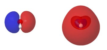
../_images/HOMO_LUMO_water.png — HOMO (left) and LUMO (right) of water.

Singly occupied molecular orbitals (SOMOs)

Singly occupied molecular orbitals (SOMOs) can be generated for radicals, and any system with unpaired electrons:

weasel example.xyz -plot-somos -mult 2

Important

SOMOs can only be generated if the molecular system contains unpaired electrons, i.e. a multiplicity of 2 (-mult 2) or higher is required.

Note

If there is more than one SOMO, the SOMOs are localized before the plots are generated.

Let us now plot the SOMOs of this 5-fold coordinated high-spin Fe(III)-heme complex.

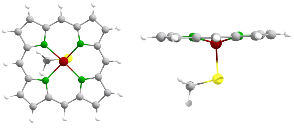
../_images/FeWAT6_struct.png — Structure of the 5-coordinate Fe(III)-heme complex.

weasel heme.xyz -mult 6 -plot-somos

After structure optimization, the SOMOs are first localized, and then plotted. We can now easily distinguish the 5 different d-orbitals of the high-spin Fe(III) complex.

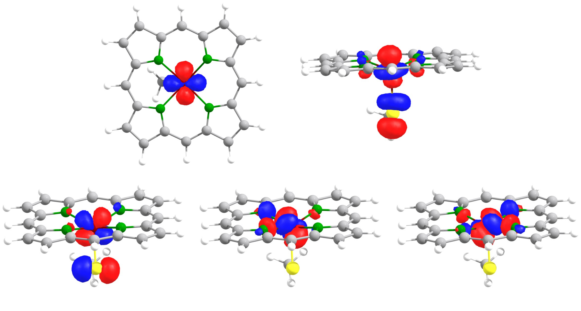
../_images/FeWAT6_MOs.png — The five SOMOs of the 5-coordinate Fe(III)-heme complex.

Note

Without the localization step before plotting, the SOMOs of the Fe(III)-heme complex would not look that textbook-like.

Spin and electron densities

The electron density (-ed) of a molecule is an observable property, describing the probability density of all its electrons summed up.

weasel structure.mol2 -plot-ed

The spin density (-sd), on the other hand, describes the probability density of the molecule's unpaired electrons.

weasel structure.mol2 -plot-sd

Keywords and remarks

Keywords for different MO and density plots:

Keyword	Description
`-plot-fmos`	Plot HOMO and LUMO, see above.
`-plot-homo`	Plot HOMO.
`-plot-lumo`	Plot LUMO.
`-plot-somos`	Plot SOMOs.
`-plot-fmos-upto INT`	Plots `INT` HOMOs and `INT` LUMOs, e.g. `-plot-fmos-upto 2`: -> generates HOMO-1, HOMO, LUMO, LUMO+1.
`-plot-mo INT1 INT2 ...`	Plots the MOs with no. `INT1`, `INT2`, and all MOs that are listed. Here, the absolute ordering of the MOs has to be known.
`-plot-ed`	Plot electron density, see below above.
`-plot-sd`	Plot spin density, see below above.

Keywords for different plotting options:

Keyword	Description
`-plot-format <options>`	Output format for plots (MO, ED, SD). Allowed <options>: `cube`, `vis`.
`-grid-res N`	Grid resolution, i.e. number of grid points per Angstrom (x, y, and z direction) for plots (MOs, ED, SD).
`-grid-x N`	Number of grid points in x direction for plots (MO, ED, SD).
`-grid-y N`	Number of grid points in y direction for plots (MO, ED, SD).
`-grid-z N`	Number of grid points in z direction for plots (MO, ED, SD).
`-grid-xmin N`	Minimum dimension on the x axis in Angstrom.
`grid-ymin N`	Minimum dimension on the y axis in Angstrom.
`-grid-zmin N`	Minimum dimension on the z axis in Angstrom.
`-grid-xmax N`	Maximum dimension on the x axis in Angstrom.
`-grid-ymax N`	Maximum dimension on the y axis in Angstrom.
`-grid-zmax N`	Maximum dimension on the z axis in Angstrom.
`-grid-xyzmin N`	Minimum dimension on x, y and z axis in Angstrom.
`-grid-xyzmax N`	Maximum dimension on x, y and z axis in Angstrom.